Introduction
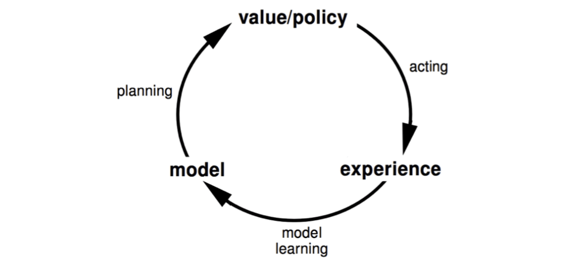
In last lecture, we learn policy directly from experience. In previous lectures, we learn value function directly from experience. In this lecture, we will learn model directly from experience and use planning to construct a value function or policy. Integrate learning and planning into a single architecture.
Model-Based RL
- Learn a model from experience
- Plan value function (and/or policy) from model
Table of Contents
Model-Based Reinforcement Learning
Advantages of Model-Based RL
- Can efficiently learn model by supervised learning methods
- Can reason about model uncertainty
Disadvantages
- First learn a model, then construct a value function -> two source of approximation error
What is a Model?
A model \(\mathcal{M}\) is a representation of an MDP \(<\mathcal{S}, \mathcal{A}, \mathcal{P}, \mathcal{R}>\) parametrized by \(\eta\).
We will assume state space \(\mathcal{S}\) and action space \(\mathcal{A}\) are known. So a model \(\mathcal{M}=<\mathcal{P}_, \eta\mathcal{R}_\eta>\) represents state transitions \(\mathcal{P}_\eta \approx \mathcal{P}\) and rewards \(\mathcal{R}_\eta\approx \mathcal{R}\). \[ S_{t+1}\sim\mathcal{P}_\eta(S_{t+1}|S_t, A_t)\\ R_{t+1}=\mathcal{R}_\eta(R_{t+1}|S_t, A_t) \] Typically assume conditional independence between state transitions and rewards.
Goal: estimate model \(\mathcal{M}_\eta\) from experience \(\{S_1, A_1, R_2, …, S_T\}\).
This is a supervised learning problem: \[ S_1, A_1 \rightarrow R_2, S_2 \\ S_2, A_2 \rightarrow R_3, S_3 \\ ...\\ S_{T-1}, A_{T-1} \rightarrow R_T, S_T \\ \] Learning \(s, a\rightarrow r\) is a regression problem; learning \(s, a\rightarrow s'\) is a density estimation problem. Pick loss function, e.g. mean-squared error, KL divergence, … Find parameters \(\eta\) that minimise empirical loss.
Examples of Models
- Table Lookup Model
- Linear Expectation Model
- Linear Gaussian Model
- Gaussian Process Model
- Deep Belief Network Model
Table Lookup Model
Model is an explicit MDP. Count visits \(N(s, a)\) to each state action pair: \[ \hat{\mathcal{P}}^a_{s,s'}=\frac{1}{N(s,a)}\sum^T_{t=1}1(S_t,A_t,S_{t+1}=s, a, s')\\ \hat{\mathcal{R}}^a_{s,s'}=\frac{1}{N(s,a)}\sum^T_{t=1}1(S_t,A_t=s, a)R_t \] Alternatively, at each time-step \(t\), record experience tuple \(<S_t, A_t, R_{t+1}, S_{t+1}>\). To sample model, randomly pick tuple matching \(<s, a, \cdot, \cdot>\).
AB Example
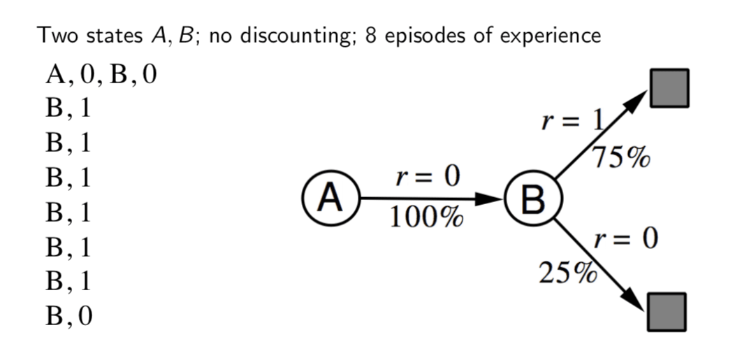
We have contrusted a table lookup model from the experience. Next step, we will planning with a model.
Planning with a model
Given a model \(\mathcal{M}_\eta=<\mathcal{P}_\eta, \mathcal{R}_\eta>\), solve the MDP \(<\mathcal{S}, \mathcal{A}, \mathcal{P}_\eta, \mathcal{R}_\eta>\) using favorite planning algorithms
- Value iteration
- Policy iteration
- Tree search
- ….
Sample-Based Planning
A simple but powerful approach to planning is to use the model only to generate samples.
Sample experience from model \[ S_{t+1}\sim\mathcal{P}_\eta(S_{t+1}|S_t,A_t)\\ R_{t+1}=\mathcal{R}_\eta(R_{t+1}|S_t,A_t) \] Apply model-free RL to samples, e.g.:
- Monte-Carlo control
- Sarsa
- Q-learning
Sample-based planning methods are often more efficient.
Back to AB Example
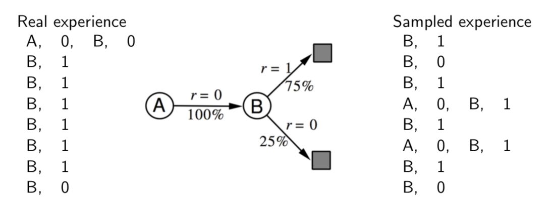
We can use our model to sample more experience and apply model-free RL to them.
Planning with an Inaccurate Model
Given an imperfect model \(<\mathcal{P}_\eta, \mathcal{R}_\eta> ≠ <\mathcal{P}, \mathcal{R}>\). Performance of model-based RL is limited to optimal policy for approximate MDP \(<\mathcal{S}, \mathcal{A}, \mathcal{P}_\eta, \mathcal{R}_\eta>\) i.e. Model-based RL is only as good as the estimated model.
When the model is inaccurate, planning process will compute a suboptimal policy.
- Solution1: when model is wrong, use model-free RL
- Solution2: reason explicitly about model uncertainty
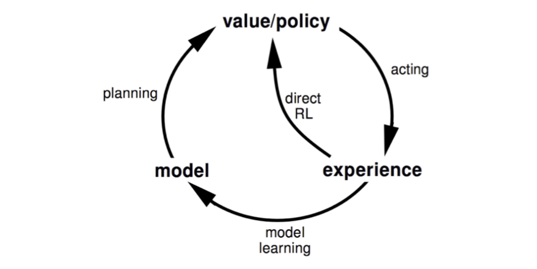
Integrated Architectures
We consider two sources of experience:
Real experience: Sampled from environment (true MDP) \[ S'\sim \mathcal{P}^a_{s,s'}\\ R=\mathcal{R}^a_s \]
Simulated experience: Sampled from model (approximate MDP) \[ S'\sim \mathcal{P}_\eta(S'|S, A)\\ R=\mathcal{R}_\eta(R|S, A) \]
Integrating Learning and Planning
Dyna Architecture
- Learn a model from real experience
- Learn and plan value function (and/or policy) from real and simulated experience
The simplest dyna algorithm is Dyna-Q Algorithm:
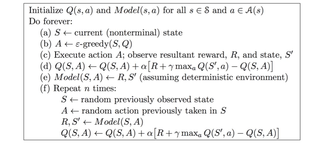
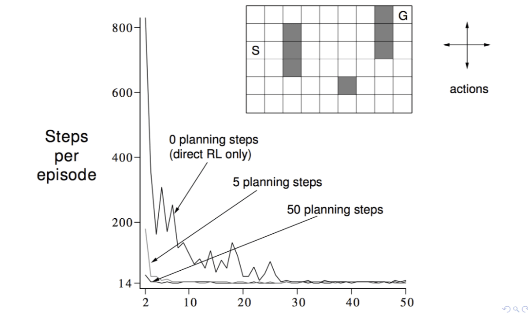
From the experiments, we can see that using planning is more efficient than direct RL only.
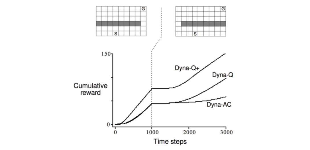
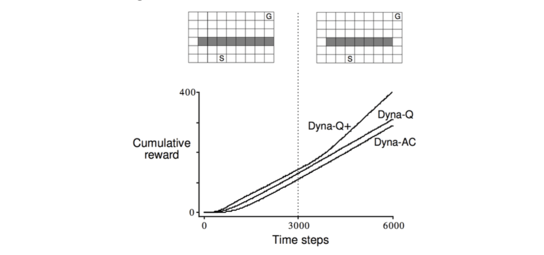
Dyna-Q with an Inaccurate Model
The changed envrionment is harder:
There is a easier change:
Simulation-Based Search
Let's back to planning problems. Simulation-based search is another approach to solve MDP.
Forward Search
Forward search algorithms select the best action by lookahead. They build a search tree with the current state \(s_t\) at the root using a model of the MDP to look ahead.
We don't need to solve the whole MDP, just sub-MDP starting from now.
Simulation-Based Search
Simulation-based search is forward search paradigm using sample-based planning. Simulate episodes of experience from now with the model. Apply model-free RL to simulated episodes.
Simulate episodes of experience from now with the model: \[ \{s_t^k, A^k_t,R^k_{t+1}, ..., S^k_T\}^K_{k=1}\sim\mathcal{M}_v \] Apply model-free RL to simulated episodes
- Monte-Carlo control \(\rightarrow\) Monte-Carlo search
- Sarsa \(\rightarrow\) TD search
Simple Monte-Carlo Search
Given a model \(\mathcal{M}_v\) and a simulation policy \(\pi\).
For each action \(a\in\mathcal{A}\)
Simulate \(K\) episodes from current (real) state \(s_t\) \[ \{s_t, a, R^k_{t+1},S^k_{t+1},A^k_{t+1}, ..., S^k_T \}^K_{k=1}\sim \mathcal{M}_v, \pi \]
Evaluate actions by mean return (Monte-Carlo evaluation) \[ Q(s_t, a)=\frac{1}{K}\sum^k_{k=1}G_t\rightarrow q_\pi(s_t, a) \]
Select current (real) action with maximum value \[ a_t=\arg\max_{a\in\mathcal{A}}Q(s_t, a) \] Monte-Carlo Tree Search
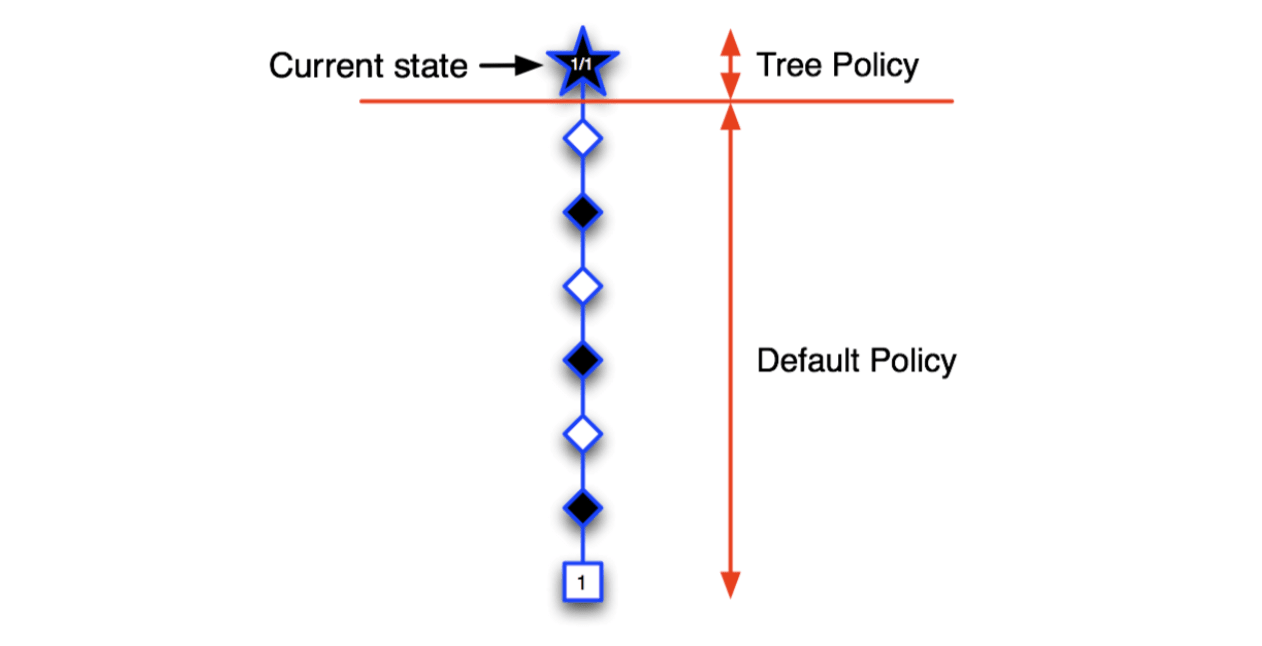
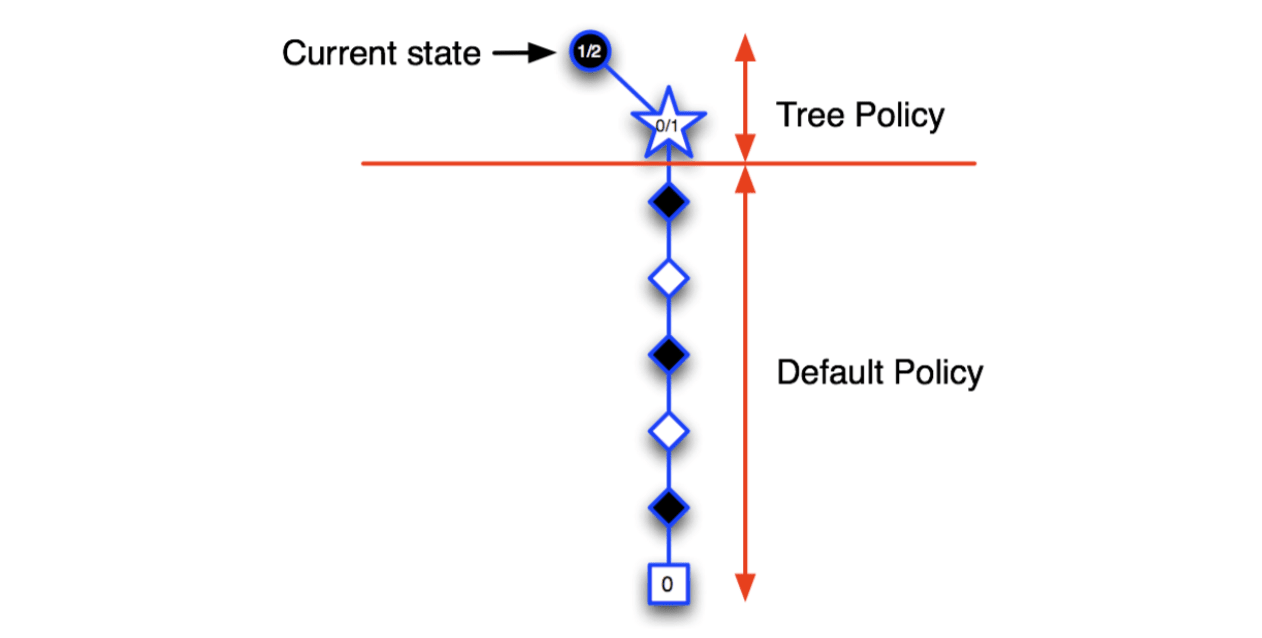
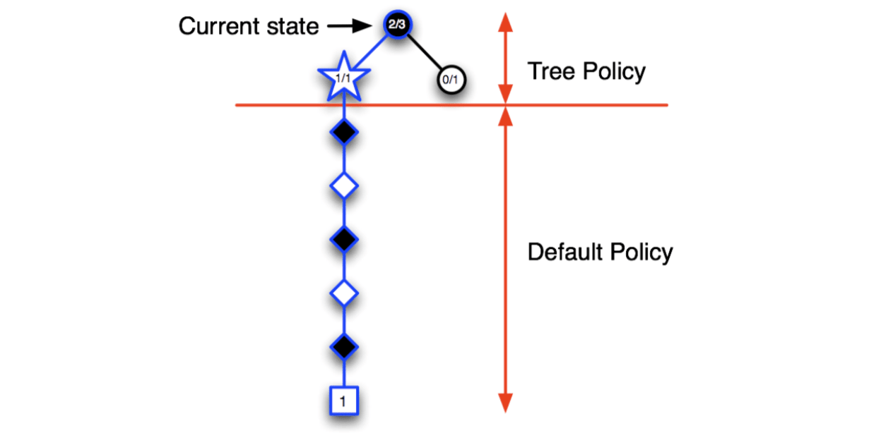
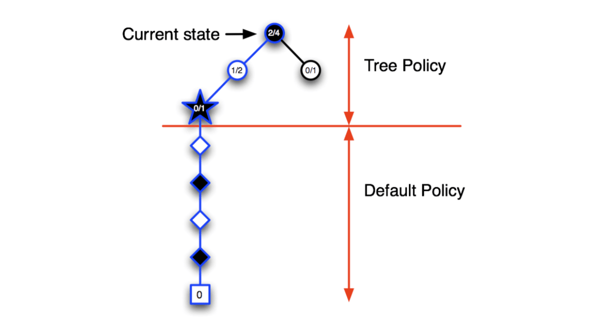
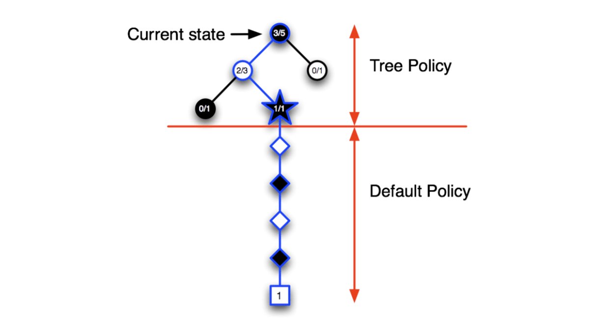
Given a model \(\mathcal{M}_v\). Simulate \(K\) episodes from current state \(s_t\) using current simulation policy \(\pi\). \[ \{s_t, A_t^k, R^k_{t+1},S^k_{t+1},A^k_{t+1}, ..., S^k_T \}^K_{k=1}\sim \mathcal{M}_v, \pi \] Build a search tree containing visited states and actions. Evaluate states \(Q(s, a)\) by mean return of episodes from \(s, a\): \[ Q(s, a)=\frac{1}{N(s,a)}\sum^K_{k=1}\sum^T_{u=t}1(S_u, A_u=s,a)G_u \to q_\pi(s,a) \] After search is finished, select current (real) action with maximum value in search tree: \[ a_t=\arg\max_{a\in\mathcal{A}}Q(s_t, a) \] In MCTS, the simulation policy \(\pi\) improves.
Each simulation consists of two phases (in-tree, out-of-tree)
- Tree policy (improves): pick actions to maximise \(Q(S,A)\)
- Default policy (fixed): pick actions randomly
Repeat (each simulation)
- \(\color{red}{\mbox{Evaluate}}\) states \(Q(S,A)\) by Monte-Carlo evaluation
- \(\color{red}{\mbox{Improve}}\) tree policy, e.g. by \(\epsilon\)-greedy(Q)
MCTS is Monte-Carlo control applied to simulated experience.
Converges on the optimal search tree, \(Q(S, A) \to q_*(S, A)\).
Case Study: the Game of Go
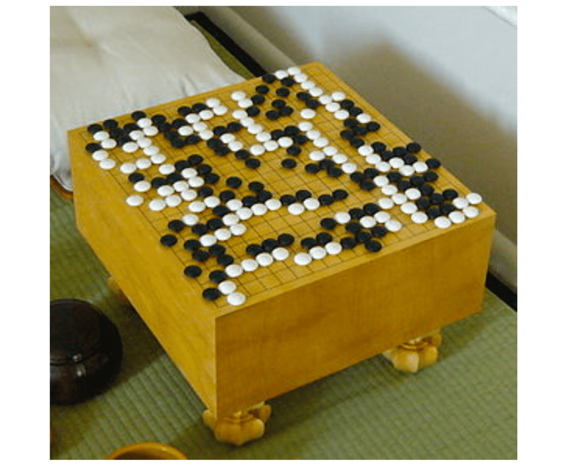
Rules of Go
- Usually played on 19$\(19, also 13\)\(13 or 9\)$9 board
- Black and white place down stones alternately
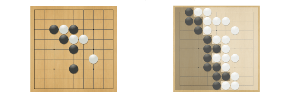
- Surrounded stones are captured and removed
- The player with more territory wins the game
Position Evaluation in Go
The key problem is how good is a position \(s\)?
So the reward function is if Black wins, the reward of the final position is 1, otherwise 0: \[ R_t = 0 \mbox{ for all non-terminal steps } t<T\\ R_T=\begin{cases} 1, & \mbox{if }\mbox{ Black wins} \\ 0, & \mbox{if }\mbox{ White wins} \end{cases} \] Policy \(\pi=<\pi_B,\pi_W>\) selects moves for both players.
Value function (how good is position \(s\)): \[ v_\pi(s)=\mathbb{E}_\pi[R_T|S=s]=\mathbb{P}[Black wins|S=s]\\ v_*(s)=\max_{\pi_B}\min_{\pi_w}v_\pi(s) \] Monte Carlo Evaluation in Go
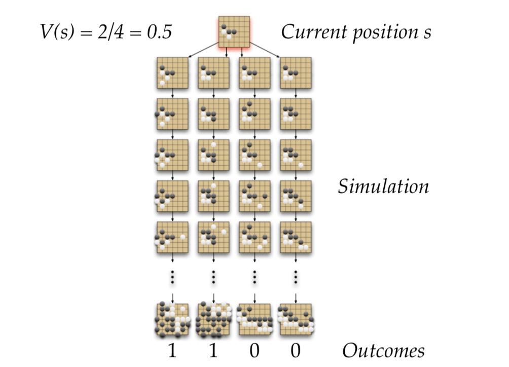
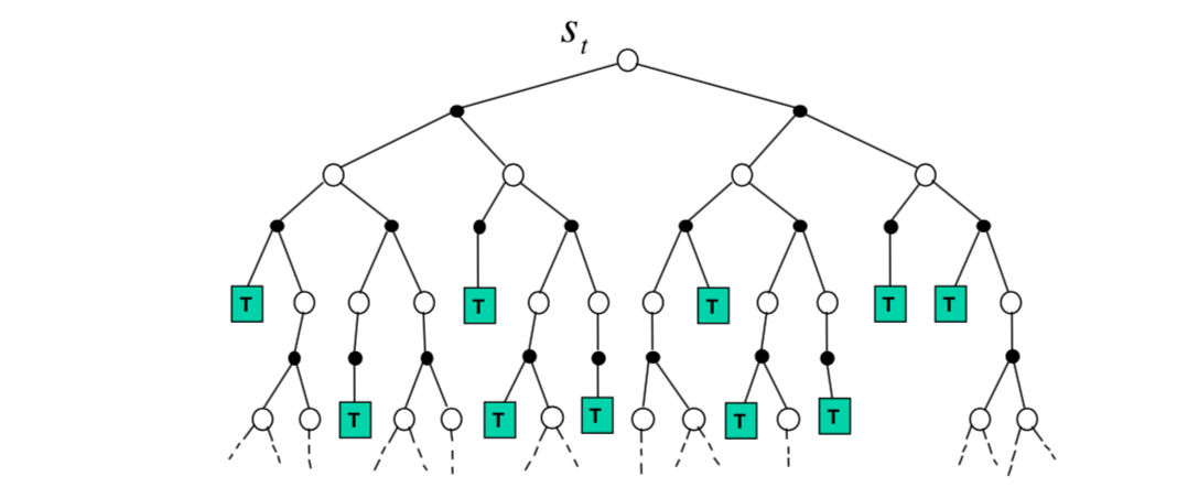
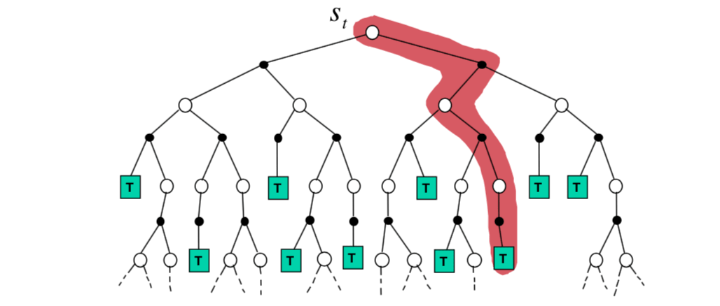
So, MCTS will expand the tree towards the node that is most promising and ignore the useless parts.
Advantages of MC Tree Search
- Highly selective best-first search
- Evaluates states dynamically
- Uses sampling to break curse of dimensionality
- Works for "black-box" models (only requires samples)
- Computationally efficient, anytime, parallelisable
Temporal-Difference Search
- Simulation-based search
- Using TD instead of MC (bootstrapping)
- MC tree search applies MC control to sub-MDP from now
- TD search applies Sarsa to sub-MDP from now
MC vs. TD search
For model-free reinforcement learning, bootstrapping is helpful
- TD learning reduces variance but increase bias
- TD learning is usually more efficient than MC
- TD(\(\lambda\)) can be much more efficient than MC
For simulation-based search, bootstrapping is also helpful
- TD search reduces variance but increase bias
- TD search is usually more efficient than MC search
- TD(\(\lambda\)) search can be much more efficient than MC search
TD Search
Simulate episodes from the current (real) state \(s_t\). Estimate action-value function \(Q(s, a)\). For each step of simulation, update action-values by Sarsa: \[ \triangle Q(S,A)=\alpha (R+\gamma Q(S',A')-Q(S,A)) \] Select actions based on action-value \(Q(s,a)\), e.g. \(\epsilon\)-greedy. May also use function approximation for \(Q\).
Dyna-2
In Dyna-2, the agent stores two sets of feature weights:
- Long-term memory
- Short-term (working) memory
Long-term memory is updated from real experience using TD learning
- General domain knowledge that applies to any episode
Short-term memory is updated from simulated experience using TD search
- Specific local knowledge about the current situation
Over value function is sum of long and short-term memories.
End.